Regular celestial images and cubes
One of the most common types of data to reproject are celestial images or n-dimensional data (such as spectral cubes) where two of the axes are celestial. There are several existing algorithms that can be used to reproject such data:
- Interpolation (such as nearest-neighbor, bilinear, biquadratic interpolation and so on). This is the fastest algorithm and is suited to common use cases, but it is important to note that it is not flux conserving, and will not return optimal results if the input and output pixel sizes are very different.
- Drizzling, which consists of determining the exact overlap fraction of pixels, and optionally allows pixels to be rescaled before reprojection. A description of the algorithm can be found in Fruchter and Hook (2002). This method is more accurate than interpolation but is only suitable for images where the field of view is small so that pixels are well approximated by rectangles in world coordinates. This is slower but more accurate than interpolation for small fields of view.
- Adaptive resampling, where care is taken to deal with differing resolutions more accurately than in simple interpolation, as described in DeForest (2004). This is more accurate than interpolation, especially when the input and output resolutions differ, or when there are strong distortions, for example for large areas of the sky or when reprojecting images that include the solar limb.
- Computing the exact overlap of pixels on the sky by treating them as four-sided spherical polygons on the sky and computing spherical polygon intersection. This is essentially an exact form of drizzling, and should be appropriate for any field of view. However, this comes at a significant performance cost. This is the algorithm used by the Montage package, and we have implemented it here using the same core algorithm. Note that this is only suitable for data being reprojected between spherical celestial coordinates on the sky that share the same origin (that is, it cannot be used to reproject from coordinates on the sky to coordinates on the surface of a spherical body).
Currently, this package implements interpolation, adaptive resampling, and spherical polygon intersection.
Note
The reprojection/resampling is always done assuming that the image is in surface brightness units. For example, if you have an image with a constant value of 1, reprojecting the image to an image with twice as high resolution will result in an image where all pixels are all 1. This limitation is due to the interpolation algorithms (the fact that interpolation can be used implicitly assumes that the pixel values can be interpolated which is only the case with surface brightness units). If you have an image in flux units, first convert it to surface brightness, then use the functions described below. In future, we will provide a convenience function to return the area of all the pixels to make it easier.
Common options
All of the reprojection algorithms implemented in reproject are available
as functions named as reproject_<algorithm>, e.g.
reproject_interp(), reproject_adaptive(),
and reproject_exact(). These can be imported from the top-level
of the package, e.g.:
>>> from reproject import reproject_interp
>>> from reproject import reproject_adaptive
>>> from reproject import reproject_exact
All functions share a common set of arguments, as well as including algorithm-dependent arguments. In this section, we take a look at the common arguments.
The reprojection functions take two main arguments. The first argument is the image to reproject, together with WCS information about the image. This can be either:
- The name of a FITS file
- An
HDUListobject - An image HDU object such as a
PrimaryHDU,ImageHDU, orCompImageHDUinstance - A tuple where the first element is a
ndarrayand the second element is either aWCSor aHeaderobject
In the case of a FITS file or an HDUList object, if
there is more than one Header-Data Unit (HDU), the hdu_in keyword argument
is also required and should be set to the ID or the name of the HDU to use.
The second argument is the WCS information for the output image, which should be
specified either as a WCS or a
Header instance. If this is specified as a
WCS instance, the shape_out keyword argument should
also be specified, and be given the shape of the output image using the Numpy
(ny, nx) convention (this is because WCS, unlike
Header, does not contain information about image
size).
As an example, we start off by opening a FITS file using Astropy:
>>> from astropy.io import fits
>>> hdu = fits.open('http://data.astropy.org/galactic_center/gc_msx_e.fits')[0]
Downloading http://data.astropy.org/galactic_center/gc_msx_e.fits [Done]
The image is currently using a Plate Carée projection:
>>> hdu.header['CTYPE1']
'GLON-CAR'
We can create a new header using a Gnomonic projection:
>>> new_header = hdu.header.copy()
>>> new_header['CTYPE1'] = 'GLON-TAN'
>>> new_header['CTYPE2'] = 'GLAT-TAN'
And finally we can call the reproject_interp() function to reproject
the image using interpolation:
>>> from reproject import reproject_interp
>>> new_image, footprint = reproject_interp(hdu, new_header)
The reprojection functions return two arrays - the first is the reprojected
input image, and the second is a ‘footprint’ array which shows the fraction of
overlap of the input image on the output image grid. This footprint is 0 for
output pixels that fall outside the input image, 1 for output pixels that fall
inside the input image. For more information about footprint arrays, see the
Footprint arrays section. To return only the main array and not the footprint,
you can set return_footprint=False.
We can then easily write out the reprojected image to a new FITS file:
>>> fits.writeto('reprojected_image.fits', new_image, new_header)
Interpolation
The reproject_interp() function can be used to carry out
reprojection implemented using simple interpolation:
>>> from reproject import reproject_interp
In addition to the arguments described in Common options, the order of the
interpolation can be controlled by setting the order= argument to either an
integer or a string giving the order of the interpolation. Supported strings
include:
'nearest-neighbor': zeroth order interpolation'bilinear': fisst order interpolation'biquadratic': second order interpolation'bicubic': third order interpolation
Adaptive resampling
The reproject_adaptive() function can be used to carry out
reprojection using the DeForest (2004) algorithm:
>>> from reproject import reproject_adaptive
In addition to the arguments described in Common options, the order of the
interpolation to use when sampling values in the input map can be controlled by
setting the order= argument to either an integer or a string giving the
order of the interpolation. Supported strings include:
'nearest-neighbor': zeroth order interpolation'bilinear': first order interpolation
Broadly speaking, the algorithm works by approximating the footprint of each output pixel by an elliptical shape in the input image which is stretched and rotated by the transformation, then finding the weighted average of samples inside that ellipse, where the weight is 1 at the center of the ellipse, and 0 at the side, and the shape of the weight function is given by an analytical distribution (currently we use a Hann function).
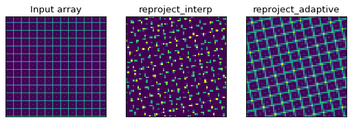
To illustrate the benefits of this method, we consider a simple case where the reprojection includes a large change in resoluton. We choose to use an artificial data example to better illustrate the differences:
import numpy as np
from astropy.wcs import WCS
import matplotlib.pyplot as plt
from reproject import reproject_interp, reproject_adaptive

# Set up initial array with pattern
input_array = np.zeros((256, 256))
input_array[::20, :] = 1
input_array[:, ::20] = 1
input_array[10::20, 10::20] = 1

# Define a simple input WCS
input_wcs = WCS(naxis=2)
input_wcs.wcs.crpix = 128.5, 128.5
input_wcs.wcs.cdelt = -0.01, 0.01

# Define a lower resolution output WCS with rotation
output_wcs = WCS(naxis=2)
output_wcs.wcs.crpix = 30.5, 30.5
output_wcs.wcs.cdelt = -0.0427, 0.0427
output_wcs.wcs.pc = [[0.8, 0.2], [-0.2, 0.8]]

# Reproject using interpolation and adaptive resampling
result_interp, _ = reproject_interp((input_array, input_wcs),
                                    output_wcs, shape_out=(60, 60))
result_deforest, _ = reproject_adaptive((input_array, input_wcs),
                                        output_wcs, shape_out=(60, 60))

plt.subplot(1, 3, 1)
plt.imshow(input_array, origin='lower', vmin=0, vmax=1, interpolation='hanning')
plt.tick_params(left=False, bottom=False, labelleft=False, labelbottom=False)
plt.title('Input array')
plt.subplot(1, 3, 2)
plt.imshow(result_interp, origin='lower', vmin=0, vmax=1)
plt.tick_params(left=False, bottom=False, labelleft=False, labelbottom=False)
plt.title('reproject_interp')
plt.subplot(1, 3, 3)
plt.imshow(result_deforest, origin='lower', vmin=0, vmax=0.5)
plt.tick_params(left=False, bottom=False, labelleft=False, labelbottom=False)
plt.title('reproject_adaptive')

In the case of interpolation, the output accuracy is poor because for each output pixel we interpolate a single position in the input array, which means that either that position falls inside a region where the flux is zero or one, and this is very sensitive to aliasing effects. For the adaptive resampling, each output pixel is formed from the weighted average of several pixels in the input, and all input pixels should contribute to the output, with no gaps.
Spherical Polygon Intersection
The reproject_exact() function can be used to carry out ‘exact’
reprojection using the spherical polygon intersection of input and output pixels:
>>> from reproject import reproject_exact
In addition to the arguments described in Common options, an optional
parallel= option can be used to control whether to parallelize the
reprojection, and if so how many cores to use (see
reproject_exact() for more details). For this algorithm, the
footprint array returned gives the exact fractional overlap of new pixels with
the original image (see Footprint arrays for more details).
Very large datasets
If you have a very large dataset to reproject, i.e., any normal IFU or radio spectral cube with many individual spectral channels - you may not be able to hold two copies of the dataset in memory. In this case, you can specify an output memory mapped array to store the data. For now this only works with the interpolation reprojection methods.
>>> outhdr = fits.Header.fromtextfile('cube_header_gal.hdr')
>>> shape = (outhdr['NAXIS3'], outhdr['NAXIS2'], outhdr['NAXIS1'])
>>> outarray = np.memmap(filename='output.np', mode='w+', shape=shape, dtype='float32')
>>> hdu = fits.open('cube_file.fits')
>>> rslt = reproject.reproject_interp(hdu, outhdr, output_array=outarray,
...                                   return_footprint=False,
...                                   independent_celestial_slices=True)
>>> newhdu = fits.PrimaryHDU(data=outarray, header=outhdr)
>>> newhdu.writeto('new_cube_file.fits')
Or if you’re dealing with FITS files, you can skip the numpy memmap step and use FITS large file creation.
>>> outhdr = fits.Header.fromtextfile('cube_header_gal.hdr')
>>> outhdr.tofile('new_cube.fits')
>>> shape = tuple(outhdr['NAXIS{0}'.format(ii)] for ii in range(1, outhdr['NAXIS']+1))
>>> with open('new_cube.fits', 'rb+') as fobj:
>>>     fobj.seek(len(outhdr.tostring()) + (np.product(shape) * np.abs(outhdr['BITPIX']//8)) - 1)
>>>     fobj.write(b'\0')
>>> outhdu = fits.open('new_cube.fits', mode='update')
>>> rslt = reproject.reproject_interp(hdu, outhdr, output_array=outhdu[0].data,
...                                   return_footprint=False,
...                                   independent_celestial_slices=True)
>>> outhdu.flush()