Available reprojection algorithms#

Overview#

There are several existing algorithms that can be used to reproject data:

Interpolation (such as nearest-neighbor, bilinear, biquadratic interpolation and so on). This is the fastest algorithm and is suited to common use cases, but it is important to note that it is not guaranteed to be photometrically accurate (see Flux/surface brightness conservation for more details about flux conservation), and will not return optimal results if the output pixels are much larger than the input pixels (since each output pixel will be the interpolated flux at one position in the input array and some input pixels will be missed altogether)
Drizzling, which consists of determining the exact overlap fraction of pixels, and optionally allows pixels to be rescaled before reprojection. A description of the algorithm can be found in Fruchter and Hook (2002). This method is more accurate than interpolation but is only suitable for images where the field of view is small so that pixels are well approximated by rectangles in world coordinates. This is slower but more accurate than interpolation for small fields of view.
Adaptive resampling, where care is taken to deal with differing resolutions more accurately than in simple interpolation, as described in DeForest (2004). This is more accurate than interpolation, especially when the input and output resolutions differ, or when there are strong distortions, for example for large areas of the sky or when reprojecting images that include the solar limb. This algorithm also applies anti-aliasing, and ultimately produces much more accurate photometry than plain interpolation. This is described in more detail in Adaptive reprojection below.
Computing the exact overlap of pixels on the sky by treating them as four-sided spherical polygons on the sky and computing spherical polygon intersection. This is essentially an exact form of drizzling, and should be appropriate for any field of view. However, this comes at a significant performance cost. This is the algorithm used by the Montage package, and we have implemented it here using the same core algorithm. Note that this is only suitable for data being reprojected between spherical celestial coordinates on the sky that share the same origin (that is, it cannot be used to reproject non-celestial coordinates or from coordinates on the sky to coordinates on the surface of a spherical body).

Currently, reproject implements all of the above except drizzling (for this you can instead use the drizzle package), and the functions to use for each are:

reproject_interp() - interpolation
reproject_adaptive() - adaptive resampling
reproject_exact() - exact overlap

If you aren’t sure what algorithm to use see Which algorithm should I use?.

Flux/surface brightness conservation#

The term ‘flux-conserving’ can be used in two different ways, and so we clarify here what we mean in the context of reproject:

The reprojection/resampling in reproject the default is to assume that the image is in surface brightness units. For example, if you have an image with a constant value of 1, reprojecting the image to an image with twice as high resolution will result in an image where all pixels are all 1. If you have an image in flux units, first convert it to surface brightness. So in this respect, the default in reproject is to preserve surface brightness, not flux.
‘Flux-conserving’ can also be used to refer not to the units specifically (flux vs surface brightness) but rather whether the output is photometrically accurate and can reliably be used to do photometry. For example, interpolation is not flux-conserving by this definition, whereas the ‘exact overlap’ method is.

We note that the adaptive resampling algorithm provides an option to conserve flux by appropriately rescaling each output pixel (see Adaptive resampling options). With this option, an image in flux units need not be converted to surface brightness - however this is not guaranteed to be photometrically flux-conserving.

Adaptive reprojection#

Broadly speaking, this algorithm works by approximating the footprint of each output pixel by an elliptical shape in the input image, which is then stretched and rotated by the transformation (as described by the Jacobian mentioned above), then finding the weighted average of samples inside that ellipse, where the shape of the weighting function is given by an analytical distribution. Hann and Gaussian functions are supported in this implementation, and this choice of functions produces an anti-aliased reprojection.

In cases where an image is being reduced in resolution, a region of the input image is averaged to produce each output pixel, while in cases where an image is being magnified, the averaging becomes a non-linear interpolation between nearby input pixels. When a reprojection enlarges some regions in the input image and shrinks other regions, this algorithm smoothly transitions between interpolation and spatial averaging as appropriate for each individual output pixel (and likewise, the amount of spatial averaging is adjusted as the scaling factor varies). This produces high-quality resampling with excellent photometric accuracy.

To illustrate the benefits of this method, we consider a case where the reprojection includes a large change in resolution. We choose to use an artificial data example to better illustrate the differences:

import numpy as np
from astropy.wcs import WCS
import matplotlib.pyplot as plt
from reproject import reproject_interp, reproject_adaptive

# Set up initial array with pattern
input_array = np.zeros((256, 256))
input_array[::20, :] = 1
input_array[:, ::20] = 1
input_array[10::20, 10::20] = 1

# Define the input WCS
input_wcs = WCS(naxis=2)
input_wcs.wcs.crpix = 128.5, 128.5
input_wcs.wcs.cdelt = -0.01, 0.01

# Define a lower resolution output WCS with rotation
output_wcs = WCS(naxis=2)
output_wcs.wcs.crpix = 30.5, 30.5
output_wcs.wcs.cdelt = -0.0427, 0.0427
output_wcs.wcs.pc = [[0.8, 0.2], [-0.2, 0.8]]

# Reproject using interpolation and adaptive resampling
result_interp, _ = reproject_interp((input_array, input_wcs),
                                    output_wcs, shape_out=(60, 60))
result_hann, _ = reproject_adaptive((input_array, input_wcs),
                                     output_wcs, shape_out=(60, 60),
                                     kernel='hann')
result_gaussian, _ = reproject_adaptive((input_array, input_wcs),
                                        output_wcs, shape_out=(60, 60),
                                        kernel='gaussian')

plt.figure(figsize=(10, 5))
plt.subplot(1, 4, 1)
plt.imshow(input_array, origin='lower', vmin=0, vmax=1, interpolation='hanning')
plt.tick_params(left=False, bottom=False, labelleft=False, labelbottom=False)
plt.title('Input array')
plt.subplot(1, 4, 2)
plt.imshow(result_interp, origin='lower', vmin=0, vmax=1)
plt.tick_params(left=False, bottom=False, labelleft=False, labelbottom=False)
plt.title('reproject_interp')
plt.subplot(1, 4, 3)
plt.imshow(result_hann, origin='lower', vmin=0, vmax=0.5)
plt.tick_params(left=False, bottom=False, labelleft=False, labelbottom=False)
plt.title('reproject_adaptive\nHann kernel')
plt.subplot(1, 4, 4)
plt.imshow(result_gaussian, origin='lower', vmin=0, vmax=0.5)
plt.tick_params(left=False, bottom=False, labelleft=False, labelbottom=False)
plt.title('reproject_adaptive\nGaussian kernel')

(png, svg, pdf)

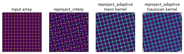
In the case of interpolation, the output accuracy is poor because, for each output pixel, we interpolate a single position in the input array which will fall inside a region where the flux is zero or one, and this is very sensitive to aliasing effects. For the adaptive resampling, each output pixel is formed from the weighted average of several pixels in the input, and all input pixels should contribute to the output, with no gaps. It can also be seen how the results differ between the Gaussian and Hann kernels. While the Gaussian kernel blurs the output image slightly, it provides much strong anti-aliasing (as the rotated grid lines appear much smoother and consistent in brightness from pixel to pixel).

Which algorithm should I use?#

Here we try and provide a few rules of thumb to help you choose the right algorithm for your use case.

First, if you are only reprojecting celestial images or the celestial slices of a higher-dimensional cube (e.g. celestial slices in a spectral cube), the origin of the coordinate system does not change between the input and the output WCS, and you need the output images to be photometrically accurate (so that you can e.g. carry out photometry on them), then use reproject_exact(). This will be slower than other methods, but is the most accurate.
If you are reprojecting data with three or more dimensions in both the input and output WCS, then reproject_interp() is the only option. This function should work on any kind of WCS (celestial or non-celestial) with any dimensionality.
If you are reprojecting images for visualization purposes (e.g. to make a plot or for a visualization tool), then reproject_interp() is usually enough.
If you need the reprojection to work well in the presence of significant distortions, including e.g. reprojecting from the surface to a body (like the Sun) to a planisphere, or if in general you want improved photometric accuracy and robustness to different input/output resolutions, use reproject_adaptive()

Note that when you have a data cube, such as a spectral cube, it is possible in principle to reproject only the celestial slices from the cube and not reproject the remaining dimension (so e.g. keep the spectral axis the same). In this case, reproject_adaptive() and reproject_exact() are valid options even though they can only handle 2-dimensional data. See Reprojecting only some dimensions of a dataset for more details.