Regular celestial images and cubes#
One of the most common types of data to reproject are celestial images or n-dimensional data (such as spectral cubes) where two of the axes are celestial. There are several existing algorithms that can be used to reproject such data:
Interpolation (such as nearest-neighbor, bilinear, biquadratic interpolation and so on). This is the fastest algorithm and is suited to common use cases, but it is important to note that it is not flux conserving, and will not return optimal results if the input and output pixel sizes are very different.
Drizzling, which consists of determining the exact overlap fraction of pixels, and optionally allows pixels to be rescaled before reprojection. A description of the algorithm can be found in Fruchter and Hook (2002). This method is more accurate than interpolation but is only suitable for images where the field of view is small so that pixels are well approximated by rectangles in world coordinates. This is slower but more accurate than interpolation for small fields of view.
Adaptive resampling, where care is taken to deal with differing resolutions more accurately than in simple interpolation, as described in DeForest (2004). This is more accurate than interpolation, especially when the input and output resolutions differ, or when there are strong distortions, for example for large areas of the sky or when reprojecting images that include the solar limb. This algorithm also applies anti-aliasing, and ultimately produces much more accurate photometry than plain interpolation.
Computing the exact overlap of pixels on the sky by treating them as four-sided spherical polygons on the sky and computing spherical polygon intersection. This is essentially an exact form of drizzling, and should be appropriate for any field of view. However, this comes at a significant performance cost. This is the algorithm used by the Montage package, and we have implemented it here using the same core algorithm. Note that this is only suitable for data being reprojected between spherical celestial coordinates on the sky that share the same origin (that is, it cannot be used to reproject from coordinates on the sky to coordinates on the surface of a spherical body).
Currently, this package implements interpolation, adaptive resampling, and spherical polygon intersection.
Note
The reprojection/resampling is always done assuming that the image is in surface brightness units. For example, if you have an image with a constant value of 1, reprojecting the image to an image with twice as high resolution will result in an image where all pixels are all 1. This limitation is due to the interpolation algorithms (the fact that interpolation can be used implicitly assumes that the pixel values can be interpolated which is only the case with surface brightness units). If you have an image in flux units, first convert it to surface brightness, then use the functions described below. In future, we will provide a convenience function to return the area of all the pixels to make it easier.
However, the adaptive resampling algorithm provides an option to conserve flux by appropriately rescaling each output pixel. With this option, an image in flux units need not be converted to surface brightness.
Common options#
All of the reprojection algorithms implemented in reproject are available
as functions named as reproject_<algorithm>, e.g.
reproject_interp(), reproject_adaptive(),
and reproject_exact(). These can be imported from the top-level
of the package, e.g.:
>>> from reproject import reproject_interp
>>> from reproject import reproject_adaptive
>>> from reproject import reproject_exact
All functions share a common set of arguments, as well as including algorithm-dependent arguments. In this section, we take a look at some of the common arguments.
The reprojection functions take two main arguments. The first argument is the image to reproject, together with WCS information about the image. This can be either:
The name of a FITS file
An
HDUListobjectAn image HDU object such as a
PrimaryHDU,ImageHDU, orCompImageHDUinstanceA tuple where the first element is a
ndarrayand the second element is either aWCSor aHeaderobject
In the case of a FITS file or an HDUList object, if
there is more than one Header-Data Unit (HDU), the hdu_in keyword argument
is also required and should be set to the ID or the name of the HDU to use.
The second argument is the WCS information for the output image, which should be
specified either as a WCS or a
Header instance. If this is specified as a
WCS instance, the shape_out keyword argument should
also be specified, and be given the shape of the output image using the Numpy
(ny, nx) convention (this is because WCS, unlike
Header, does not contain information about image
size).
As an example, we start off by opening a FITS file using Astropy:
>>> from astropy.io import fits
>>> hdu = fits.open('http://data.astropy.org/galactic_center/gc_msx_e.fits')[0]
Downloading http://data.astropy.org/galactic_center/gc_msx_e.fits [Done]
The image is currently using a Plate Carée projection:
>>> hdu.header['CTYPE1']
'GLON-CAR'
We can create a new header using a Gnomonic projection:
>>> new_header = hdu.header.copy()
>>> new_header['CTYPE1'] = 'GLON-TAN'
>>> new_header['CTYPE2'] = 'GLAT-TAN'
And finally we can call the reproject_interp() function to reproject
the image using interpolation:
>>> from reproject import reproject_interp
>>> new_image, footprint = reproject_interp(hdu, new_header)
The reprojection functions return two arrays - the first is the reprojected
input image, and the second is a ‘footprint’ array which shows the fraction of
overlap of the input image on the output image grid. This footprint is 0 for
output pixels that fall outside the input image, 1 for output pixels that fall
inside the input image. For more information about footprint arrays, see the
Footprint arrays section. To return only the main array and not the footprint,
you can set return_footprint=False.
We can then easily write out the reprojected image to a new FITS file:
>>> fits.writeto('reprojected_image.fits', new_image, new_header)
Interpolation#
The reproject_interp() function can be used to carry out
reprojection implemented using simple interpolation:
>>> from reproject import reproject_interp
In addition to the arguments described in Common options, the order of the
interpolation can be controlled by setting the order= argument to either an
integer or a string giving the order of the interpolation. Supported strings
include:
'nearest-neighbor': zeroth order interpolation'bilinear': first order interpolation'biquadratic': second order interpolation'bicubic': third order interpolation
Adaptive resampling#
The reproject_adaptive() function can be used to carry out
anti-aliased reprojection using the DeForest (2004) algorithm:
>>> from reproject import reproject_adaptive
This algorithm provides high-quality photometry through anti-aliased reprojection, which avoids the problems of plain interpolation when the input and output images have different resolutions, and it offers a flux-conserving mode.
Options#
In addition to the arguments described in Common options, one can use the options described below.
A rescaling of output pixel values to conserve flux can be enabled with the
conserve_flux flag. (Flux conservation is stronger with a Gaussian
kernel—see below.)
The kernel used for interpolation and averaging can be controlled with a set of
options. The kernel argument can be set to ‘hann’ or ‘gaussian’ to set the
function being used. The Gaussian window is the default, as it provides better
anti-aliasing and photometric accuracy (or flux conservation, when the
flux-conserving mode is enabled), though at the cost of blurring the output
image by a few pixels. The kernel_width argument sets the width of the
Gaussian kernel, in pixels, and is ignored for the Hann window. This width is
measured between the Gaussian’s \(\pm 1 \sigma\) points. The default value
is 1.3 for the Gaussian, chosen to minimize blurring without compromising
accuracy. Lower values may introduce photometric errors or leave input pixels
under-sampled, while larger values may improve anti-aliasing behavior but will
increase blurring of the output image. Since the Gaussian function has infinite
extent, it must be truncated. This is done by sampling within a region of
finite size. The width in pixels of the sampling region is determined by the
coordinate transform and scaled by the sample_region_width option, and this
scaling represents a trade-off between accuracy and computation speed. The
default value of 4 represents a reasonable choice, with errors in extreme cases
typically limited to less than one percent, while a value of 5 typically reduces
extreme errors to a fraction of a percent. (The sample_region_width option
has no effect for the Hann window, as that window does not have infinite
extent.)
One can control the calculation of the Jacobian used in this
algorithm with the center_jacobian flag. The Jacobian matrix represents
how the corresponding input-image coordinate varies as you move between output
pixels (or d(input image coordinate) / d(output image coordinate)), and serves
as a local linearization of the coordinate transformation. When this flag is
True, the Jacobian is calculated at pixel grid points by calculating the
transformation at locations offset by half a pixel, and then doing finite
differences on the resulting input-image coordinates. This is more accurate but
carries the cost of tripling the number of coordinate transformed done by this
routine. This is recommended if your coordinate transform varies significantly
and non-smoothly between output pixels. When False, the Jacobian is
calculated using the pixel-grid-point transforms that need to be computed
anyway, which produces Jacobian values at locations between pixel grid points,
and nearby Jacobian values are averaged to produce values at the pixel grid
points. This is more efficient, and the loss of accuracy is extremely small for
transformations that vary smoothly between pixels. The default (False) is
to use the faster option.
In some situations (e.g. an all-sky map, with a wrap point in the longitude),
extremely large Jacobian values may be computed which are artifacts of the
coordinate system definition, rather than reflecting the actual nature of the
coordinate transformation. This may result in a band of nan pixels in the
output image. In these situations, if the actual transformation is
approximately constant in the region of these artifacts, the
despike_jacobian option should be enabled. If enabled, the typical
magnitude (distance from the determinant) of the Jacobian matrix, Jmag2 =
sum_j sum_i (J_ij**2), is computed for each pixel and compared to the 25th
percentile of that value in the local 3x3 neighborhood (i.e. the third-lowest
value). If it exceeds that percentile value by more than 10 times, the Jacobian
matrix is deemed to be “spiking” and it is replaced by the average of the
non-spiking values in the 3x3 neighborhood.
When, for any one output pixel, the sampling region in the input image
straddles the boundary of the input image or lies entirely outside the input
image, a range of boundary modes can be applied, and this is set with the
boundary_mode option. Allowed values are:
strict— Output pixels will beNaNif any of their input samples fall outside the input image.constant— Samples outside the bounds of the input image are replaced by a constant value, set with theboundary_fill_valueargument. Output values becomeNaNif there are no valid input samples.grid-constant— Samples outside the bounds of the input image are replaced by a constant value, set with theboundary_fill_valueargument. Output values will beboundary_fill_valueif there are no valid input samples.ignore— Samples outside the input image are simply ignored, contributing neither to the output value nor the sum-of-weights normalization. If there are no valid input samples, the output value will beNaN.ignore_threshold— Acts asignore, unless the total weight that would have been assigned to the ignored samples exceeds a set fraction of the total weight across the entire sampling region, set by theboundary_ignore_thresholdargument. In that case, acts asstrict.nearest— Samples outside the input image are replaced by the nearest in-bounds input pixel.
The input image can also be marked as being cyclic or periodic in the x and/or
y axes with the x_cyclic and y_cyclic flags. If these are set, samples
will wrap around to the opposite side of the image, ignoring the
boundary_mode for that axis.
This implementation includes several options for handling nan and inf
values in the input data, set via the bad_value_mode argument:
strict— Values ofnanorinfin the input data are propagated to every output value which samples them.ignore— When a sampled input value isnanorinf, that input pixel is ignored (affected neither the accumulated sum of weighted samples nor the accumulated sum of weights).constant— Input values ofnanandinfare replaced with a constant value, set via thebad_fill_valueargument.
Algorithm Description#
Broadly speaking, the algorithm works by approximating the footprint of each output pixel by an elliptical shape in the input image, which is then stretched and rotated by the transformation (as described by the Jacobian mentioned above), then finding the weighted average of samples inside that ellipse, where the shape of the weighting function is given by an analytical distribution. Hann and Gaussian functions are supported in this implementation, and this choice of functions produces an anti-aliased reprojection. In cases where an image is being reduced in resolution, a region of the input image is averaged to produce each output pixel, while in cases where an image is being magnified, the averaging becomes a non-linear interpolation between nearby input pixels. When a reprojection enlarges some regions in the input image and shrinks other regions, this algorithm smoothly transitions between interpolation and spatial averaging as appropriate for each individual output pixel (and likewise, the amount of spatial averaging is adjusted as the scaling factor varies). This produces high-quality resampling with excellent photometric accuracy.
To illustrate the benefits of this method, we consider a simple case where the reprojection includes a large change in resolution. We choose to use an artificial data example to better illustrate the differences:
import numpy as np
from astropy.wcs import WCS
import matplotlib.pyplot as plt
from reproject import reproject_interp, reproject_adaptive

# Set up initial array with pattern
input_array = np.zeros((256, 256))
input_array[::20, :] = 1
input_array[:, ::20] = 1
input_array[10::20, 10::20] = 1

# Define a simple input WCS
input_wcs = WCS(naxis=2)
input_wcs.wcs.crpix = 128.5, 128.5
input_wcs.wcs.cdelt = -0.01, 0.01

# Define a lower resolution output WCS with rotation
output_wcs = WCS(naxis=2)
output_wcs.wcs.crpix = 30.5, 30.5
output_wcs.wcs.cdelt = -0.0427, 0.0427
output_wcs.wcs.pc = [[0.8, 0.2], [-0.2, 0.8]]

# Reproject using interpolation and adaptive resampling
result_interp, _ = reproject_interp((input_array, input_wcs),
                                    output_wcs, shape_out=(60, 60))
result_hann, _ = reproject_adaptive((input_array, input_wcs),
                                     output_wcs, shape_out=(60, 60),
                                     kernel='hann')
result_gaussian, _ = reproject_adaptive((input_array, input_wcs),
                                        output_wcs, shape_out=(60, 60),
                                        kernel='gaussian')

plt.figure(figsize=(10, 5))
plt.subplot(1, 4, 1)
plt.imshow(input_array, origin='lower', vmin=0, vmax=1, interpolation='hanning')
plt.tick_params(left=False, bottom=False, labelleft=False, labelbottom=False)
plt.title('Input array')
plt.subplot(1, 4, 2)
plt.imshow(result_interp, origin='lower', vmin=0, vmax=1)
plt.tick_params(left=False, bottom=False, labelleft=False, labelbottom=False)
plt.title('reproject_interp')
plt.subplot(1, 4, 3)
plt.imshow(result_hann, origin='lower', vmin=0, vmax=0.5)
plt.tick_params(left=False, bottom=False, labelleft=False, labelbottom=False)
plt.title('reproject_adaptive\nHann kernel')
plt.subplot(1, 4, 4)
plt.imshow(result_gaussian, origin='lower', vmin=0, vmax=0.5)
plt.tick_params(left=False, bottom=False, labelleft=False, labelbottom=False)
plt.title('reproject_adaptive\nGaussian kernel')
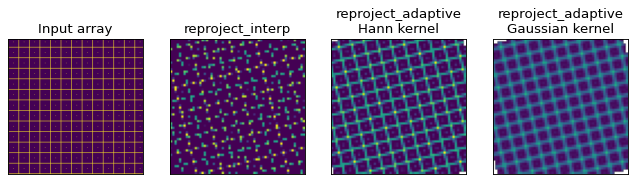
In the case of interpolation, the output accuracy is poor because, for each output pixel, we interpolate a single position in the input array which will fall inside a region where the flux is zero or one, and this is very sensitive to aliasing effects. For the adaptive resampling, each output pixel is formed from the weighted average of several pixels in the input, and all input pixels should contribute to the output, with no gaps. It can also be seen how the results differ between the Gaussian and Hann kernels. While the Gaussian kernel blurs the output image slightly, it provides much strong anti-aliasing (as the rotated grid lines appear much smoother and consistent in brightness from pixel to pixel).
Spherical Polygon Intersection#
The reproject_exact() function can be used to carry out ‘exact’
reprojection using the spherical polygon intersection of input and output pixels:
>>> from reproject import reproject_exact
For this algorithm, the footprint array returned gives the exact fractional overlap of new pixels with the original image (see Footprint arrays for more details).
Warning
The reproject_exact() is currently known to
have precision issues for images with resolutions <0.05”. For
now it is therefore best to avoid using it with such images.