Combining images into mosaics#
Warning
The mosaicking functionality in the reproject package is currently experimental, so use with care and please report issues at astropy/reproject
The reproject.mosaicking sub-package includes helper functions for
constructing mosaics from multiple images. These are
find_optimal_celestial_wcs(), which can be used to
construct a single optimal WCS/shape that overlaps with multiple images, and
reproject_and_coadd(), which given images and a
target WCS/shape will reproject all the images then combine them into a mosaic.
We describe these in the sections below.
For the examples on this page we will use the PyVO module to retrieve tiles from the 2MASS survey around the M17 region:
>>> from astropy.io import fits
>>> from astropy.coordinates import SkyCoord
>>> from pyvo.dal import imagesearch
>>> pos = SkyCoord.from_name('M17')
>>> table = imagesearch('https://irsa.ipac.caltech.edu/cgi-bin/2MASS/IM/nph-im_sia?type=at&ds=asky&',
...                    pos, size=0.25).to_table()
>>> table = table[(table['band'].astype('S') == 'K') & (table['format'].astype('S') == 'image/fits')]
>>> m17_hdus =  [fits.open(url)[0] for url in table['download'].astype('S')]
Computing an optimal WCS#
Basic usage#
Given a series of images, the
find_optimal_celestial_wcs() function can be
used to find an output WCS and shape (i.e. an output header) that overlaps with
all the inpute images. Note that you don’t necessarily need to use this if you
already know the final header or WCS you want to use for the images - in this
case you can skip straight to Reprojecting and co-adding images into a mosaic.
You can optionally provide options to try and constrain
the solution, as we will see below. To start off, let’s consider the simplest
example, which is to call find_optimal_celestial_wcs()
with the files downloaded above, but no additional information:
>>> from reproject.mosaicking import find_optimal_celestial_wcs
>>> wcs_out, shape_out = find_optimal_celestial_wcs(m17_hdus)
The first argument to find_optimal_celestial_wcs()
should be a list where each element is either a filename, an HDU object (e.g.
PrimaryHDU or ImageHDU), an
HDUList object, or a tuple of (array, wcs). In the
example above, we have passed a list of HDUs. We can now look at the output
WCS and shape:
>>> wcs_out.to_header()
WCSAXES =                    2 / Number of coordinate axes
CRPIX1  =      900.07981909504 / Pixel coordinate of reference point
CRPIX2  =      1099.9484609446 / Pixel coordinate of reference point
CDELT1  =     -0.0002777777845 / [deg] Coordinate increment at reference point
CDELT2  =      0.0002777777845 / [deg] Coordinate increment at reference point
CUNIT1  = 'deg'                / Units of coordinate increment and value
CUNIT2  = 'deg'                / Units of coordinate increment and value
CTYPE1  = 'RA---TAN'           / Right ascension, gnomonic projection
CTYPE2  = 'DEC--TAN'           / Declination, gnomonic projection
CRVAL1  =      275.18472258448 / [deg] Coordinate value at reference point
CRVAL2  =     -16.141349044263 / [deg] Coordinate value at reference point
LONPOLE =                180.0 / [deg] Native longitude of celestial pole
LATPOLE =     -16.141349044263 / [deg] Native latitude of celestial pole
...
>>> shape_out
(2201, 1800)
Coordinate system#
By default, the coordinate system of the first file is used, and the final
WCS is set up so that North (in that coordinate system) is up. In the
case above, the images are in equatorial coordinates, so the final WCS is also
in equatorial coordinates. We can force the output WCS to instead be in
Galactic coordinates by setting the frame= argument to a coordinate frame
object such as Galactic or one of the string
shortcuts defined in astropy (e.g. 'fk5', 'galactic', etc.):
>>> wcs_out, shape_out = find_optimal_celestial_wcs(m17_hdus,
...                                                 frame='galactic')
the resulting WCS is then in Galactic coordinates:
.. doctest-requires:: pyvo
>>> wcs_out.to_header()
WCSAXES =                    2 / Number of coordinate axes
CRPIX1  =      1214.1034417971 / Pixel coordinate of reference point
CRPIX2  =      1310.1351675461 / Pixel coordinate of reference point
CDELT1  =     -0.0002777777845 / [deg] Coordinate increment at reference point
CDELT2  =      0.0002777777845 / [deg] Coordinate increment at reference point
CUNIT1  = 'deg'                / Units of coordinate increment and value
CUNIT2  = 'deg'                / Units of coordinate increment and value
CTYPE1  = 'GLON-TAN'           / galactic longitude, gnomonic projection
CTYPE2  = 'GLAT-TAN'           / galactic latitude, gnomonic projection
CRVAL1  =      15.116960053834 / [deg] Coordinate value at reference point
CRVAL2  =    -0.72166403860488 / [deg] Coordinate value at reference point
LONPOLE =                180.0 / [deg] Native longitude of celestial pole
LATPOLE =    -0.72166403860488 / [deg] Native latitude of celestial pole
...
>>> shape_out
(2623, 2424)
Orientation#
As mentioned above, by default the image will be lined up so that North is up,
but this may not always be optimal because if the mosaic is rotated compared to
North, there may be a lot of empty space in the final mosaic. The auto_rotate
option can therefore be used to find the optimal rotation for the WCS that minimizes
the area of the final mosaic file:
>>> wcs_out, shape_out = find_optimal_celestial_wcs(m17_hdus,
...                                                 frame='galactic',
...                                                 auto_rotate=True)
Note that this requires Shapely 1.6 or later to be installed. We can now look at the final WCS and shape:
>>> wcs_out.to_header()
WCSAXES =                    2 / Number of coordinate axes
CRPIX1  =      1102.3949574309 / Pixel coordinate of reference point
CRPIX2  =      900.46211361965 / Pixel coordinate of reference point
PC1_1   =     0.88188439264557 / Coordinate transformation matrix element
PC1_2   =     0.47146571244169 / Coordinate transformation matrix element
PC2_1   =    -0.47146571244169 / Coordinate transformation matrix element
PC2_2   =     0.88188439264557 / Coordinate transformation matrix element
CDELT1  =     -0.0002777777845 / [deg] Coordinate increment at reference point
CDELT2  =      0.0002777777845 / [deg] Coordinate increment at reference point
CUNIT1  = 'deg'                / Units of coordinate increment and value
CUNIT2  = 'deg'                / Units of coordinate increment and value
CTYPE1  = 'GLON-TAN'           / galactic longitude, gnomonic projection
CTYPE2  = 'GLAT-TAN'           / galactic latitude, gnomonic projection
CRVAL1  =      15.116960053834 / [deg] Coordinate value at reference point
CRVAL2  =    -0.72166403860488 / [deg] Coordinate value at reference point
LONPOLE =                180.0 / [deg] Native longitude of celestial pole
LATPOLE =    -0.72166403860488 / [deg] Native latitude of celestial pole
...
>>> shape_out
(1800, 2201)
As expected, the optimal shape is smaller than was returned previously.
Pixel resolution#
By default, the final mosaic will have the pixel resolution (i.e. the pixel
scale along the pixel axes) of the highest resolution input image, but this can
be overridden using the resolution= keyword argument:
>>> from astropy import units as u
>>> wcs_out, shape_out = find_optimal_celestial_wcs(m17_hdus,
...                                                 resolution=1.5 * u.arcsec)
Projection and reference coordinate#
Finally, you can customize the projection to use as well as the reference
coordinate. To change the projection from the default (which is the
gnomonic projection, or TAN), you can use the projection= keyword
argument, which should be set to a valid three-letter FITS-WCS projection
code:
>>> wcs_out, shape_out = find_optimal_celestial_wcs(m17_hdus,
...                                                 projection='CAR')
To customize the reference coordinate (where the projection is centered) you
can set the reference= keyword argument to an astropy
SkyCoord object:
>>> from astropy.coordinates import SkyCoord
>>> coord = SkyCoord.from_name('M17')
>>> wcs_out, shape_out = find_optimal_celestial_wcs(m17_hdus,
...                                                 reference=coord)
Reprojecting and co-adding images into a mosaic#
Assuming that you have a set of images that you want to combine into a mosaic,
as well as a target header or WCS and shape (which you either determined
independently, or with Computing an optimal WCS), you can make use of the
reproject_and_coadd() function to produce the
mosaic:
>>> from reproject import reproject_interp
>>> from reproject.mosaicking import reproject_and_coadd
>>> array, footprint = reproject_and_coadd(m17_hdus,
...                                        wcs_out, shape_out=shape_out,
...                                        reproject_function=reproject_interp)
The first argument to reproject_and_coadd()
should be a list where each element is either a filename, an HDU object (e.g.
PrimaryHDU or ImageHDU), an
HDUList object, or a tuple of (array, wcs).
The second argument is the WCS information for the output image, which should
be specified either as a WCS or a
Header instance. If this is specified as a
WCS instance, the shape_out argument to
reproject_interp() should also be specified, and be
given the shape of the output image using the Numpy (ny, nx) convention
(this is because WCS, unlike
Header, does not contain information about image
size).
Finally, the reproject_function should be used to specify which function to
use to reproject individual tiles - this should be either
reproject_interp() or reproject_exact() - with
the latter being slower but more accurate (and necessary for flux conservation).
Keyword arguments for these functions (e.g. order for
reproject_interp()) can be passed as keyword arguments to
reproject_and_coadd().
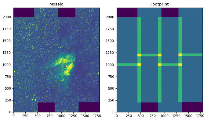
The example above will return an array which is the mosaic itself, and a footprint, which shows how many input images contributed to each output pixel. We can take a look at the output:
import numpy as np
import matplotlib.pyplot as plt

plt.figure(figsize=(10, 8))
ax1 = plt.subplot(1, 2, 1)
im1 = ax1.imshow(array, origin='lower', vmin=600, vmax=800)
ax1.set_title('Mosaic')
ax2 = plt.subplot(1, 2, 2)
im2 = ax2.imshow(footprint, origin='lower')
ax2.set_title('Footprint')
In some cases, including the above example, each tile that was used to compute
the mosaic has an arbitrary offset due e.g. to different observing conditions.
The reproject_and_coadd() includes an option to
match the backgrounds (assuming a constant additive offset in each image):
>>> array_bgmatch, _ = reproject_and_coadd(m17_hdus,
...                                        wcs_out, shape_out=shape_out,
...                                        reproject_function=reproject_interp,
...                                        match_background=True)
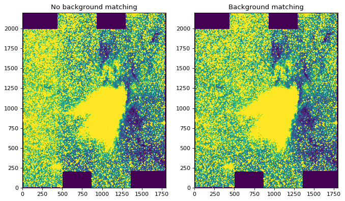
By adjusting the stretch, we can see the difference more clearly between the mosaic made with background matching and that made without - the one without shows vertical striping, especially on the left.
import numpy as np
import matplotlib.pyplot as plt

ax1 = plt.subplot(1, 2, 1)
im1 = ax1.imshow(array, origin='lower', vmin=635, vmax=660)
ax1.set_title('No background matching')
ax2 = plt.subplot(1, 2, 2)
im2 = ax2.imshow(array_bgmatch, origin='lower', vmin=635, vmax=660)
ax2.set_title('Background matching')
The background matching works by finding all overlapping pairs of images and determining the median difference for each pair, then using a stochastic gradient descent method to find the optimal additive corrections (a positive or negative constant for each image) to minimize differences. We additionally place the constraint that the average correction should be zero, but since there’s no reason that the average correction should be exactly zero, you should be aware that the final mosaic may be offset from the absolute surface brightness/flux by a constant additive factor. The algorithm should be robust for many situations and does not currently have any exposed options for fine tuning.